
I developed lecture notes for Control Systems awhile back when I was the Chair of the Department of Computer Engineering at the University of San Carlos. And this one is part of the lecture/lab notes.
Objective
To introduced MATLAB Basic commands and its many different toolboxes which could be used in this course.
Introduction
MATLAB is an interactive program for numerical computation and data visualization; it is used extensively by many fields for analysis and design. There are many different toolboxes available which extend the basic functionality of MATLAB into different application areas. Additional information of this software can be found on www.mathworks.com
Running MATLAB
Find the shortcut icon of MATLAB located in your computer desktop. Double click and wait for awhile to load the MATLAB Command Prompt. You will see the Figure 1.1 on your desktop once MATLAB already finished loading,
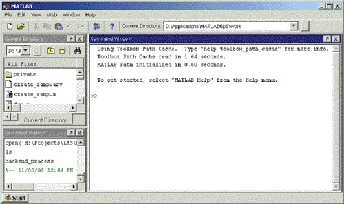
Figure 1.1 MATLAB Command Prompt
The “double greater than sign” (>>) is the command prompt of MATLAB. This is where you need to type in your MATLAB commands.
Vectors in MATLAB
Creating vectors in MATLAB is quite straightforward. To create a vector, one need only to define a variable, which you normally do in any programming language, assign some values to that variable, but in this case, the coefficients. For example, to create a vector x, follow this command in the MATLAB prompt.
>>
Once you type in this command MATLAB will return the following:
It is easy also to create a vector with elements that are evenly spaced. For instance, let us create a vector y, which has elements from 15 to 50 and evenly spaced in increments of 10. Syntax: variable = start : increment : end
>>
MATLAB will return the following:
Vector Manipulation
It is also straightforward to manipulate vectors in MATLAB. Suppose, one wants to add something to each of the elements in a vector x. Just follow this sample command:
>>
MATLAB will return:
To add or subtract vectors together, you need only to used this command
>> a = b + c
>> a = b – c
Note however, that vectors that are added or subtracted should have the same dimensions. This means that if you have a 4 elements vector, the other vectors should also have 4 elements on it, otherwise you will have an error of dimension mismatch. (Matrix dimensions must agree.)
Functions in MATLAB
MATLAB includes a lot of standard functions. Each of these functions is a block of code that accomplishes a specific task. This functions has the same meaning in a programming languages that you have studied, for instance, the clrscr() in Turbo C, or the classes in your java subjects. Some of these functions include but is not limited only to the one mention below:
Trigonometric Functions, e.g., sin, cos, and etc.
Mathematical Functions, e.g., log, exp, sqrt and etc.
Commonly used constants, e.g., pi, i, and j.
For example:
>> sin(pi/2)
MATLAB returns:
ans =
1
Note that on this example, ans was automatically created since you did not specify any variable that will hold your immediate answer. These means that you can also used ans as variable. Note also that these value/s will change once there will be new commands typed in the prompt that does not have any assigned variables.
To get more information on the syntax of any function, Type at the MATLAB command prompt (sometimes referred to as command window),
>> help function name
For example:
>> help sin
MATLAB returns:
SIN Sine.
SIN(X) is the sine of the elements of X.
See also asin, sind.
Overloaded functions or methods (ones with the same name in other directories)
help sym/sin.m
Reference page in Help browser
doc sin
How to make a graphical representation in MATLAB
To plot a trigonometric function in MATLAB, type this in your command prompt,
>> time = 0:0.1:5
As was discussed earlier, you simply create a vector from 0 to 5 with 0.1 increment. You will see that after you typed in this command, there will be about 51 columns for this one, and you will see that each of this column have a 0.1 differences to its neighboring values. Now, type the next command and press enter after each line:
>> fx=sin(time)
>> plot(time,fx)
After the third command typed, there is another window that will be open which creates the plot of sin() with respect to your time variable.
Notice that in each of the first two commands, you saw a lot of values that has been displayed. We can suppress these values, by ending these first two commands with semi-colon (;). For instance,
>> time=0:0.1:5;
>> fx=sin(time);
>> plot(time,fx)
On Polynomials in MATLAB
Polynomial in MATLAB is being represented by a vector. Since we already have presented on how to represent vectors in MATLAB, then it will be very easy to represent polynomials. Each of the element that we describe earlier in vectors is actually the coefficients of the polynomials. We need only to enter each of these elements in descending order. For example, suppose we have this polynomial:
It’s MATLAB equivalent command will be:
>> x=[25 2 0 -5]
MATLAB returns:
x =
25 2 0 -5
Note that the “0” in one of the element represent the ‘s’ part of the polynomial. Since the degree of the polynomial is 3 then, there will be an expected of 4 coefficients, thus your description of variable x. Generally, an nth order polynomial will have n+1 number of coefficients (vector length). So, if we have this polynomial,
Your MATLAB declaration should be:
>> x=[1 0 0 0 0 -25]
We can evaluate polynomials by using the function – polyval().
>> polyval(x,2)
ans =
7
To extract the roots of a polynomial is easy. Used the roots() function. For example,
>> roots(x)
ans =
-1.5401 + 1.1189i
-1.5401 – 1.1189i
0.5883 + 1.8105i
0.5883 – 1.8105i
1.9037
Multiplying two polynomials can also be done by using the convolution of their coefficients. Note that the product of two polynomials is equivalent to the convolution of their coefficients. Use conv() function.
>> poly1=[1 2 3];
>> poly2=[4 5 6 7];
>> prod=conv(poly1,poly2)
prod =
4 13 28 34 32 21
To divide two polynomials, you only need to used the deconv() function. Note that the return value consists of two parts, one is the quotient and the other is the remainder. As an example, let’s use the variable prod and poly2, and will try to checked if indeed the result will give us poly1.
>>deconv(prod,poly2)
ans =
1 2 3
You’ve noticed that since the result does not have any remainder thus, it did not display it for this example.
If you are interested in getting the polynomial of a given roots, it can be done using the poly([roots]) functions. Suppose we have a simpler function given by,
(s+3)(s+4) = ?
To find its compact form,
>> poly([ -3 -4])
ans =
1 7 12
Therefore
(Missing equation here – will try to check later on how to display equation in HTML)
Matrices in MATLAB
To create a matrix in MATLAB, is the same as creating a vector, with the exception that, each row is separated by a semi-colon (;) or by an Enter key (You need to press the Enter Key of course.). For example,
>> B=[1 2 3;4 5 6;7 8 9]
B =
1 2 3
4 5 6
7 8 9
or you can do this,
>> B=[1 2 3
4 5 6
7 8 9]
B =
1 2 3
4 5 6
7 8 9
As we all knew that we can manipulate matrix, e.g., taking the transpose, performing mathematical operations on two matrices and etc. You have to be very careful in taking the product of two matrices, commutative property does not apply, thus,
To find the transpose of a matrix in MATLAB, use an apostrophe after the matrix variable. For example, in reference to the matrix define above, matrix B,
>>transB=B’
If one wants to multiply two matrix element by element, you only need to used the “.*” (dot-asterisk) operator. The two matrices must have the same size.
For example
>> MatrixA=[1 2;3 4];
>> MatrixB=[2 1;4 3];
>> MatrixA.*MatrixB
Raising the power of a square matrix can also be done using MATLAB by using the “^” operator. For example,
>> MatrixA^3
ans =
37 54
81 118
In the case that you need only to raise the power of each element, then used the dot operator.
>> MatrixA.^2
ans =
1 4
9 16
To find the inverse of a matrix and its eigenvalues using the following commands respectively, inv() and eig().
>> inv(MatrixA)
ans =
-2.0000 1.0000
1.5000 -0.5000
Running group of commands automatically
MATLAB files usually have an extension of “m”. For example, plotsine.m. Thus in order to organize your files, you should always remember to put an extension to all your MATLAB files. This will facilitate in easy searching and if you would follow the proper filenaming convention, you don’t even need to open the file, but you will know exactly what it is for by just its name. Thus, from now, for example, if you have a group of commands that plots a sine function. It would be advisable to save that group of commands to a file name that best reflects its functionality for instance, plotsine.m, or sineplot.m.
As an example of grouping of commands and saving it in an m-file, try creating the plotsine.m and store all the necessary commands in it (See – How to make a graphical representation in MATLAB). You can use notepad or any other IDE to enter the three commands and save the file as txt/ascii.
Then, once saved, try to load it in the MATLAB command prompt:
>> plotsine
This will give you a plot, same as the plot that we generated before, but without the hassle of putting/typing all the required commands.
You can either type commands directly into MATLAB, or put all of the commands that you will need together in an m-file, and just run the file. If you put all of your m-files in the same directory that you run MATLAB from, then MATLAB will always find them.
MATLAB’s “Eject-Button”
MATLAB as with other programming/script languages has a good on-line help. Try typing this in the MATLAB command prompt.
Help command
Getting more information on the command as long as you know what particular command you are asking for additional information.